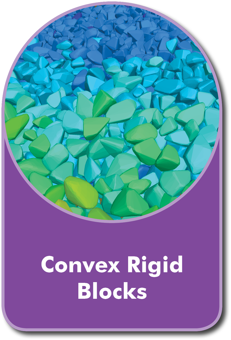
You can now model convex rigid polygons (2D) and polyhedra (3D). This allows modeling of non-spherical objects when the shape is of importance (granular or cohesive systems) without requiring clumps. Contact detection and resolution use a variation of the GJK (Gilbert–Johnson–Keerthi) algorithm with only one contact between two objects (i.e., no sub-contacts) to maximize efficiency. Interactions between rigid blocks and between other PFC components, such as balls, clumps, or walls, are possible using regular contact models. Similar to balls and clumps (PFC) and blocks (UDEC/3DEC), a fully dynamic solution scheme is employed.
Convex rigid block utilities include:
- Easy shape creation
- Shape import shape from CAD data
- Automatic computation of convex shape from a set of vertices
- Replication or generation of multiple blocks from templates (similar to clumps)
- Cutting existing blocks into smaller ones (stochastically or deterministically)
- Filtering blocks by aspect ratio or relative volume during cutting to remove slivers
- Merging blocks
- Rounding edges and corners to reduce the number of active contacts
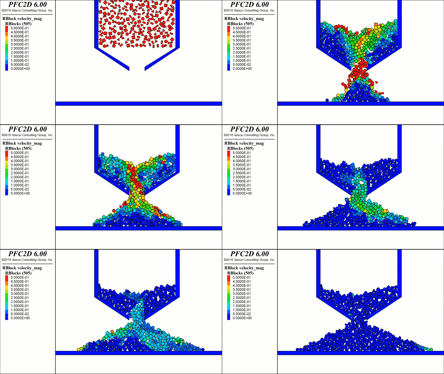
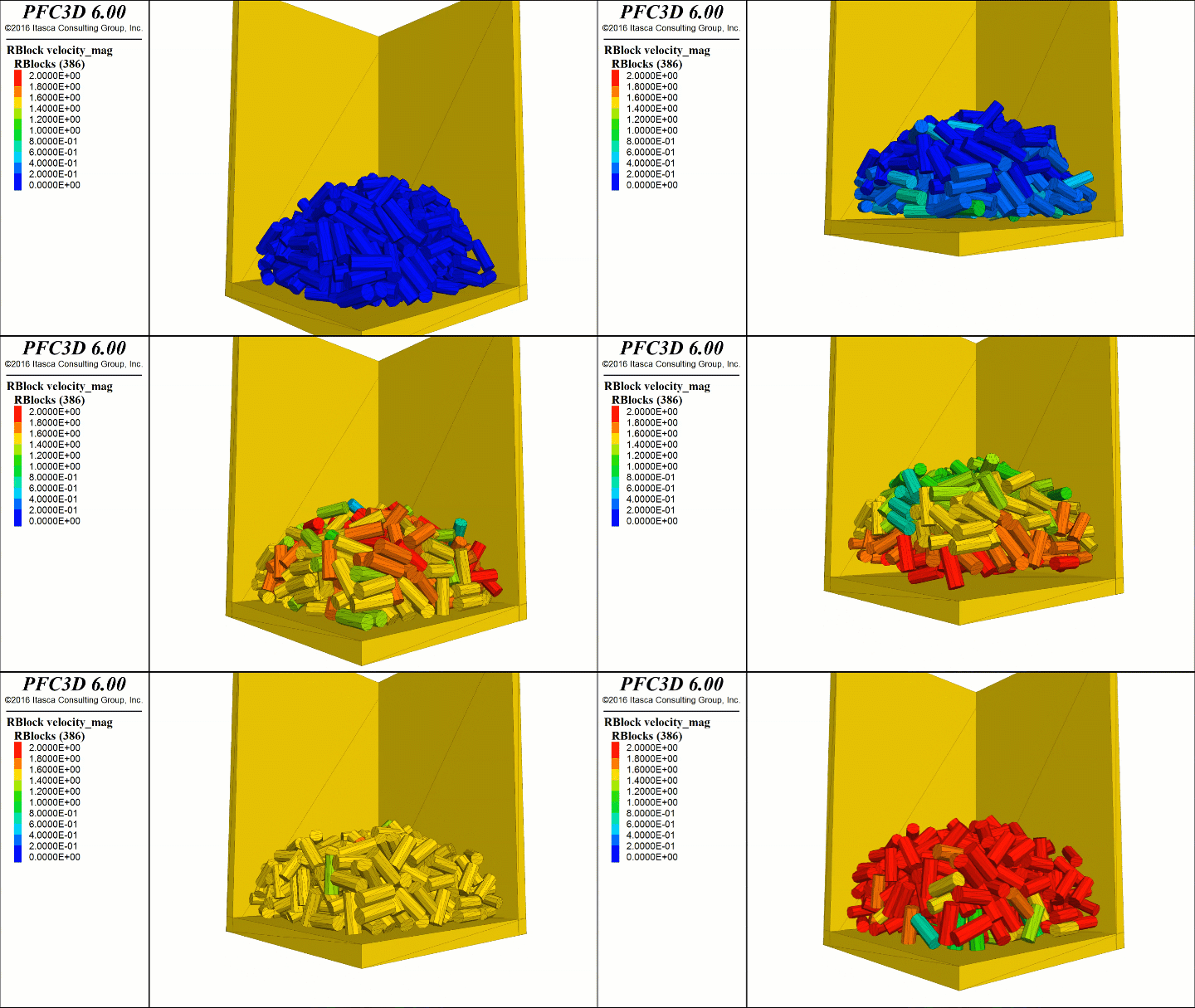
The following rigid block examples show contours of block velocity for a bin flow example (left) and cylindrical blocks undergoing mixing through shaking (right).
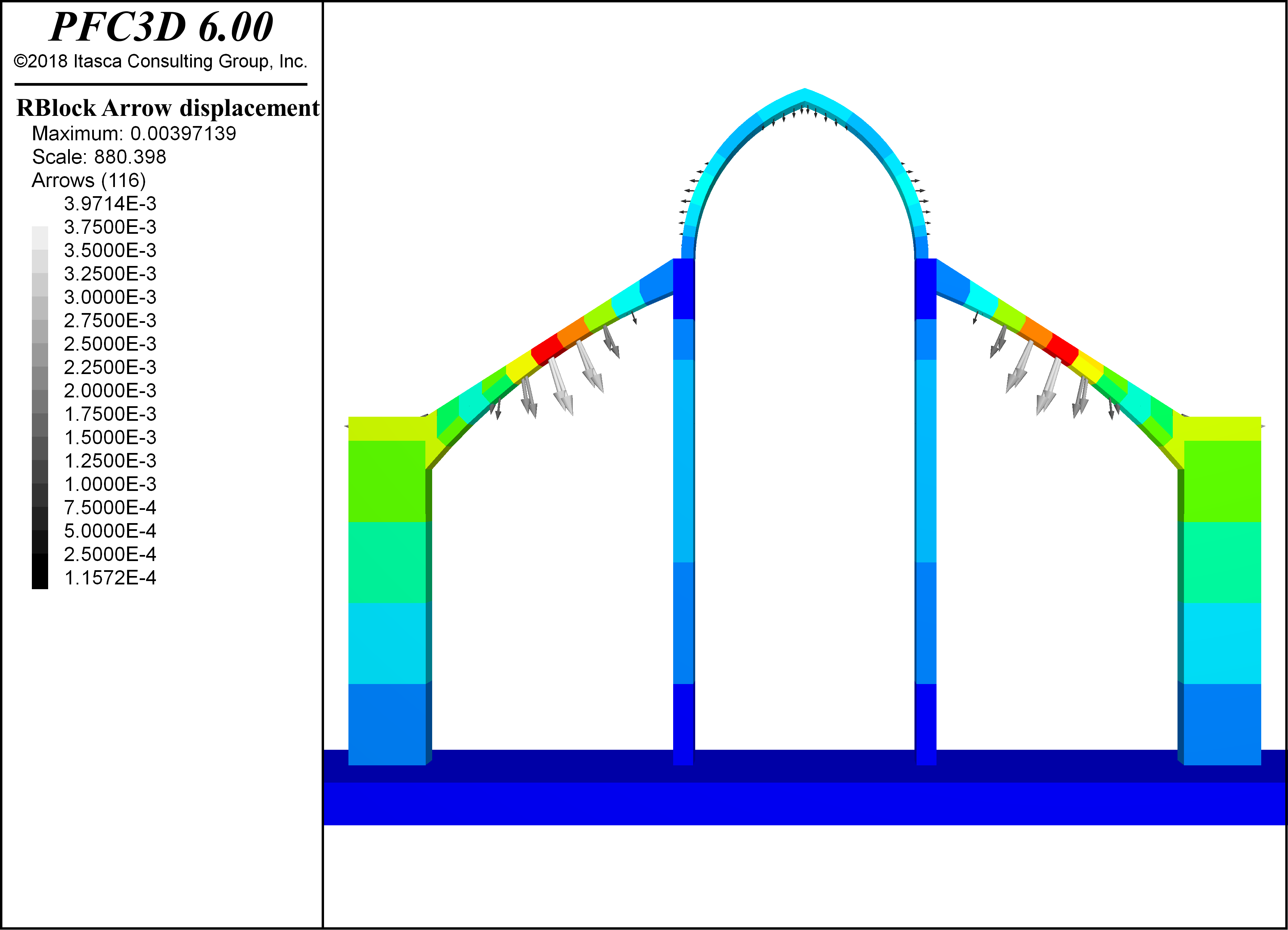
The next illustration is based on a 3DEC model that demonstrates the effectiveness of flying buttresses in a supporting a thin-walled arch. The structure is simulated as a collection of rigid blocks and the deformation under gravity loading is observed. The model is run with (left) and without (right) buttresses to examine their effect.
Bonded Block Models (BBM)
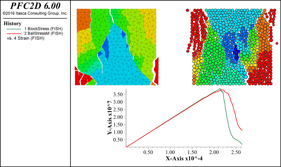
In addition to granular and cohesive systems, now it is easy to create bonded block models (BBM) similar to UDEC and 3DEC. For example, the following compares a PFC2D BBM (left) with a conventional PFC2D bonded particle model (BPM) undergoing a simulated unconfined, uniaxial compression test. The two model plots indicate sample damage and fragmentation. An xy chart of Axial Stress vs. Axial Strain is shown below the two model samples.
